Get Complete Project Material File(s) Now! »
Above the threshold : intermittency and spatial correlations
In experiments a mean velocity v > 0 is often imposed to the interface. This is the most realistic way to trigger several avalanches in a finite amount of time. Hence the system is above the critical point and the transition is approached by making v as small as possible. In this case the line never completely stops and subsequents avalanches are triggered before the previous ones stop. This complicates the task of defining avalanches without ambiguity.
For a finite system, when v is very small, v ! 0+, the instantaneous velocity v(t) of the center of mass is very intermittent : it is very large for short period and very low for longer periods. The mean velocity v is the time average of the instantaneous velocity v(t). A standard procedure to define the avalanches is to threshold the velocity signal of the center-of-mass of the interface : avalanches are defined as the periods where v(t) exceeds a threshold vth. The duration T of the avalanche is the time period where v(t) stays above vth and the avalanche size S is the integral of the difference between the signal and the threshold over this period (see figure 1.3a). However this kind of analysis raises important issues : if the threshold is too large, a single avalanche may be interpreted as a series of seemingly distinct events, while if it is too small subsequent avalanches can be merged into a single event [14, 15]. Furthermore it does not take into account the spatial fluctuations of the velocity (a portion of the interface can be moving fast while other portions stay pinned) and local events can be skipped. Hence disentangling avalanches and accurately measuring critical exponents are a major challenge. In chapter 3 I will propose an alternative method to determine the critical exponents, which is based on the correlations of the local velocity signal.
In figure 1.3b I show the velocities of two points that are close to each other along the line in a crack propagation experiment [4]. We see that they are intermittent, as is the center-of-mass velocity. We also see that the two points move fast or slow roughly at the same time : there are spatial correlations in the system. The motion of the interface occurs through the motion of correlated domains. These domains have a maximal size that diverges as f approaches fc from above as : (f − fc)− .
Scaling relations between exponents
In section 1.1 I introduced exponents characterizing the depinning transition. As for equilibrium phase transitions we can establish relations between the exponents using scaling arguments. In this section I derive four relations, leaving only two independents exponents out of six.
From equations (1.1.8), (1.1.9) v scales as −/. From (1.1.1) and (1.1.6) the mean velocity inside an avalanche of extension ` scales as `−z. Making the assumption that the mean velocity inside the largest avalanches (of extension ) is proportional to the mean velocity of the interface we can say that v −z and we have the first relation : = (z − ) . (1.4.1). Sizes and durations are defined for each avalanche. Because they are defined for the same events and scale together the probability laws are equal : P(S)dS = P(T)dT . Inserting the scaling relation (1.1.7) in the power-regime of the equality we can write T− T −1dT T−˜dT with = (d + )/z. This yields the second relation : = d + z = ˜ − 1 − 1 . (1.4.2). The last two relations derive from a symmetry of the problem called Statistical Tilt Symmetry.
The Barkhausen noise
When slowly varying the magnetic field through a piece of ferromagnetic material such as iron, the magnetization in the material changes and generates ”irregular induction pulses in a coil wound around the sample, that can then be heard as a noise in a telephone” [39] (and [40] for a translation in english of the original article). This noise, recorded for the first time by Heinrich Barkhausen in 1919 [39], is nowadays known as the Barkhausen noise or the Barkhausen effect. Barkhausen originally assumed that the noise was created by flipping magnets. It was the first evidence of the existence of the magnetic domains postulated by Pierre-Ernest Weiss in 1906. However in 1949 it was evidenced that the jumps in the magnetization were actually related to the irregular motion of the domain walls (DWs) between domains of opposite magnetization [40, 41]1. Domain walls are visible in figure 2.1a which shows an image of magnetic domains in a ferromagnetic alloy. Figure 2.2a shows a sketch of an experimental setup used to record the Barkhausen noise. A ferromagnetic material is put in the center of a solenoid. A current in the solenoid generates in its center a uniform magnetic field, hereafter called external field. This field induces a magnetization of the sample which in turn induces a response magnetic field. A pickup coil wounded around the sample detects the induced magnetic flux . Figure 2.2b shows the magnetic flux change ˙ = @t in two different samples and for different oscillation frequencies of the applied field. The applied signal is triangular in order to have a constant growth rate of the external field during the measurement. When the driving rate is high the signal is constituted of intertwinned overlapping pulses. At low driving rate the pulses become well separated in time and one can define Barkhausen jumps as the events when the signal exceeds some small threshold. This jumps have a given size S and duration T (defined in figure 1.3a)which are power law distributed with exponents and ˜ : P(S) S− , P(T) T−˜ .
Crack front propagation
Crackling noise can also be recorded during the failure of brittle heterogeneous materials under slow external loading. Here the crackling signal refers to the mean crack speed and its variation with time. In this section I briefly describe two experiments that provide a direct observation of an in-plane crack propagation. The first one, originally performed by J. Schmittbuhl and K.J. M°aløy in 1997, is a reference experiment in the crack field and is coloquially known as ”the Oslo experiment” [52]. The second one, designed by J. Chopin and L. Ponson, is directly inspired by the former but slightly different. To differentiate it from the first one I refer to it as ”d’Alembert experiment”, because it was performed at Institut d’Alembert in Paris. I analyzed the data issued from this experiment and the results I obtained are presented in chapter 3 and in the publication [4].
Oslo experiment The setup consists of two transparent plates of Plexiglas annealed together at 200C and several bars of pressure. The annealed surface is a plane of weaker toughness. Before annealing defects are introduced by sandblasting the surfaces with steel particles of 50μm diameter [52]. This introduces random flucutations in the toughness of the weak plane. Then a crack is opened by pulling apart the two plates (so called Mode I crack, see figure 2.3a). It propagates along the weak plane of the annealed surface. Pictures of the system are taken with a digital camera mounted on a microscope. The crack front appears as the interface between a clear and a dark region on the image (as can be seen on the bottom picture of figure 2.4 taken on the d’Alembert experiment). The direct observation of the front allowed to measure the roughness exponent . The first measurements yield values in the range = − 0.50 − 0.66 [52, 53]. This is at variance with the predictions of the model. The crack front is expected to be described by an elastic string with the long-range kernel (1.2.9) with = 1 [54]. For this model the roughness exponent has been estimated very precisely by a numerical method which give the value = 0.388±0.002 [31]. The discrepancy was resolved in 2010 when it was found that the value − actually describes the roughness of the front at short scales and that crossovers to + 0.35 − 0.37 at large scales [55]. The crossover is governed by the Larkin length [56] below which the Larkin model predicts a roughness exponent L = − d/2 = 0.5 (cf. equation (1.3.5)) consistent with the experimental results.
Wetting of disordered susbtrates
When a liquid is dropped on a solid substrate it can either spread and form a film that covers the solid (total wetting) or form a meniscus (partial wetting). In the latter case, the line where the liquid surface meets the solid is called contact line, wetting front or triple line. It has been shown independently by Joanny and de Gennes [2] and by Pomeau and Vannimenus [64] that the contact line can be described as an elastic line with long-range elasticity arising from the surface tension of the meniscus. In this section I reproduce the computation from Joanny and de Gennes of the elastic energy associated to a small deformation of the line, as it is useful to understand the assumptions under which the form of the elastic energy holds (this has also been done in the PhD Thesis [38]). Then I present an experiment and discuss results about the roughness exponent.
Elastoplasticity and the yielding transition
In the depinning transition, an elastic interface starts to flow above a finite force threshold fc. A behavior that is similar in many respects is shared by some amorphous solids. In contrast to crystalline solids, amorphous solids have no internal structure. Typical exemples of such materials are foams, mayonnaise or whipped cream. When left at rest they are solids : they do not flow and keep their initial shape. But one can make them flow easily by applying a sufficiently large shear stress, in which case they behave more like liquids. See [86] for a recent review on the deformation and flow of amorphous solids. As for the depinning the onset of the flow arises at a finite value of the stress, called yield stress because the solid yields. These materials are named yield stress solids and the transition from solid to liquid behaviour is called the yielding transition.
The deformation of the solid under the shear stress occurs through local shear transformations (also named plastic events) where the particles rearrange locally. This rearrangement reduces the local stress which is redistributed elastically in the rest of the material. The redistributed stress can trigger new plastic events, possibly leading to an avalanche of plastic events and a macroscopic deformation of the material.
Formally the local deformation from the initial configuration is measured by the local plastic strain (x), where x 2 Rd is the internal coordinate of the solid. It can be seen as a d-dimensional interface in d+1 dimension, as illustrated in figure 2.9. As the depinning, the yielding transition is characterized by a set of critical exponents characterizing a diverging length scale, the avalanche size distribution or the strain rate versus stress curve (see right of figure 2.9 for the latter). The dynamics of the plastic strain is governed by : @t (x) = +Z G(x − y) (y) + dis x, (x) .
Table of contents :
Introduction
1 Disordered elastic systems and the depinning transition
1.1 Phenomenology of the depinning transition
1.2 Equation of motion
1.3 The Larkin length and the upper critical dimension
1.4 Scaling relations between exponents
1.5 Middleton theorems
1.6 Conclusion
2 Experimental realisations
2.1 The Barkhausen noise
2.2 Crack front propagation
2.3 Wetting of disordered susbtrates
2.4 Earthquakes
2.5 Elastoplasticity and the yielding transition
2.6 Conclusion
3 Assessing the Universality Class of the transition
3.1 Existing methods to characterize the transition
3.2 A novel method based on the universal scaling of the local velocity field
3.3 Conjecture for the correlation functions in plasticity
3.4 Conclusion
4 Cluster Statistics
4.1 Introduction of the observables and various critical exponents
4.2 Recall of previous results
4.3 Cluster statistics
4.4 Statistics of gaps and avalanche diameter
4.5 Tables of exponents
4.6 Conclusion
5 Mean-Field models
5.1 What is mean-field ?
5.2 Fully-connected and ABBM models
5.3 Introduction of the Brownian force model
5.4 Insights into the long-range instanton equation with a local source
5.5 Conclusion
Summary and perspectives
Appendix
A Fourier transform of the elastic force
B Computation of the elastic coefficients for numerical simulations
C Analysis of the experimental data
D Computation of the generating functional using the Martin-Siggia-Rose formalism
Bibliography