Get Complete Project Material File(s) Now! »
Global Imbalances with Safe Assets in a Monetary Union
Abstract
In a two-country economy with the stochastic mean-variance output process, the safe assets help the consumers to attain the full risk-sharing across the domestic and foreign risky investments. A higher domestic productivity level raises both the mean and variance of the domestic output, and can lead to a greater accumulation of the safe assets. The empirical analysis on the 19 countries of Eurozone confirms this theoretical implication. Moreover, it also reveals that the accumulation of the safe assets is the main driver of the global imbalances in Eurozone.
Introduction
The global imbalances in Eurozone are featured by three stylized facts.
Fact 1: The net total capital inflows for each country have been increasing from 1990s (when the European Economic Area is established to allow the free move-ment of capital across countries) and have boosted up substantially from 2000s when the introduction of one common currency.
Fact 2: Both exporters and importers of capital are the advanced economies. The panel A in Figure 2.1.1 shows that Germany, Netherlands and Austria are the main exporters of capital while France, Italy, Spain are the main importers of capitals. This flow of capital from developed to developed economies is different to the up-hill capital flows from developing to developed economies (Lucas para-dox).
Fact 3: The Debt flows dominate the FDI and Portfolio flows on shaping the pat-tern of capital flows across countries. The panel B demonstrates that the negative of net total capital inflows is driven mainly by the negative of net debt inflows for Germany. This structure of capital flows is the same for Spain (Panel C).
Despite a large body of literature on global imbalances for last decades, there are a few formal structures to analyze the case of Eurozone. On many models, capital can flow out from developing countries with the severe financial friction. Both creditors and debtors in Eurozone, however, do not differ by level of financial friction (Panel A). Some models argue that the advanced economies can have the valuation gains on the international investment position due to the exchange rate fluctuation and differential rate of returns on foreign assets and liabilities. The same currency in Eurozone, however, rules out the effect of the exchange rate on the international investment position. Furthermore, the dominant role of bonds on shaping the pattern of capital flows has not been explored yet (Panel B and C).
The main purpose of this paper is to provide a framework of endogenous portfo-lio choice to analyze the international capital flows when both foreign assets and liabilities are denominated into one common currency. We stresses the role of the safe assets on shaping the pattern of capital flows. We use this model to show that the dominant features in Figure 2.1.1 can arise from the interaction between the productivity level and the available supply of the safe asset.
We decompose the net total capital inflows into the flows of the risky investments (FDI and Portfolio) and the risk-free Bonds. To generate the heterogeneity rate of return on the risky assets across countries, the productivity level is allowed to be different across countries. To analyze the demand for risk-free bonds, we employ a mean-variance output growth process with the risk-averse agents. With an AK production function, a higher productivity level raises both the mean and variance of the rate of return on the risky investment, and motivates the agents to hold the safe asset to insure against the high variance in the risky investments. With these key features, the model sheds light on the motivation behind the flows of both the risky and the risk-free investments across countries with the similar economic fundamentals.
Next, we carry out the empirical analysis on one panel data from Eurostat on 19 countries in Eurozone. The empirical result strongly supports that a higher pro-ductivity level results in a greater accumulation of foreign bonds. The empirical test using the data from Alfaro, Kalemli-Ozcan and Volosovych (2014) provides the same result.
The paper offers a theory of the international capital flows across countries in one monetary union. Past papers on the current account adjustment in Eurozone rely on the low saving and high investment rates due to convergence in output per capita (Blanchard and Giavazzi (2002)), on the convergence and growth expec-tations (Lane and Pels (2012)), on the allocation of imported capital between tradable and non-tradable sectors (Giavazzi and Spaventa (2011)). Some dis-tinguishing elements mark our theory from the aforementioned papers. First, we separate the risky investments’ flows (FDI and portfolio) to the risk-free invest-ments’ flows (bonds) by allowing the agents to hold a rich portfolio choice including both risky and safe assets. Second, we emphasize the change of net foreign assets rather than the conventional current account to account for the role of the real unexpected capital gains on shaping the cross-border capital flows. Third, we ap-proach the global imbalances with a balance between the theory and the empirical analysis.
Our paper is related to the literature on the role of the safe asset on the global economy. Farhi and Maggiori (2016) focus on the competition on supplying the safe asset as the key element on the architectrure of the international monetary system. Farhi, Caballero and Gourinchas (2008) argue the high supply of the fi-nancial assets in advanced economies helps them to attract net total capital flows from developing economies. He, Krishnamurthy and Milbradt (2016) character-ize the safe assets based on the float of the sovereign bonds and the fundamentals available to rollover the public debt. Taking the supply side as given, we focus on the demand side of safe assets to shed light on the pattern of international capital flows across countries. Within a mean-variance production process, an increase of productivity can lead to a greater accumulation of the safe asset if the agent is risk averse enough.
Our work is also related to the growing theoretical macro-finance literature that incorporates endogenous portfolio choice into models of open economy macroecon-omy, such as with the asymmetric information (Tille and Wincoop (2010), home bias on equity (Coeurdacier and Rey (2013)). These papers provide a various approximation technique to analyze current account around the steady state. Our paper produces an exact closed-form characterization of the equilibrium. This feature is familiar with Pavlova and Rigobon (2010a)’s pure-exchange economy. Our model, however, shuts down the price adjustment process and elaborates one open production economy with more general utility function.
The paper proceeds as follows. Section 2.2 describes the economic environment and characterizes the equilibrium. Section 2.3 focuses on the role of safe assets. Section 2.4 analyzes the international capital flows. Section 2.5 presents the em-pirical evidence to support the theory. Section 2.6 concludes and the appendix presents two extended models.
The model
The economic setting
We work with a continuous-time production economy populated by two countries: Home and Foreign. Home is the core economy with a higher productivity level than Foreign as the periphery one: a > a∗.
Technology
Both countries produce one common free mobile good which can be consumed or accumulated as capital and traded in a perfectly integrated world capital market. The flows of outputs at Home (dy) and at Foreign (dy∗) are produced by means of the stochastic linear production functions, using domestic domiciled capitals
dy = akdt + akσdz (2.1)
dy∗ = a∗k∗dt + a∗k∗σ∗dz∗ (2.2)
where (a, k); (a∗, k∗) are productivity levels and capital stocks in Home and For-eign respectively. The parameters (σ; σ∗) are non-negative constants, representing the variance. The terms (dz; dz∗) represent the proportional productivity shocks in Home and Foreign. The set-up features the mean-variance analysis (Turnovsky (1997)) to address important trade-offs between the level of macroeconomic per-formance and the associated risks. z and z∗ are Wiener processes with the increments that are normally distributed with zero mean (E[dz] = E[dz∗] = 0) and variance (E[dz2] = E[dz∗2] = dt). The productivity shock is assumed to be country-specific: Cov(dz, dz∗) = 0.
Beside the two risky assets, there are also the risk-free Bonds which we call the safe assets. The supply of safe assets is exogenous so that the safe interest rate is endogenous determined. The exogeneity of safe assets supply can be intepreted as the monetary union, as a whole, can borrow from the rest of world. The main reason is that, technically, since both Home and Foreign agents have the same risk averse coefficient, there is no motivation for one economy to issue the safe assets (risk-free Bonds) to the other. And the model of endogenous supply of safe assets need to rely on the heterogeneity of risk averse coefficient (Farhi and Maggiori (2016)). The exogenous supply of the safe assets, therefore, is necessary to assure the market clearing conditions. This feature is also the key on Farhi, Caballero and Gourinchas (2008) in which the supply of safe assets is a constant fraction of domestic output. In the Appendix, we present two alternative models which incorporate the heterogenity on the risk aversion and on the supply of safe assets across countries. These two alternative models, however, are more appropriate to capture the global imbalance between two blocks of economies: advanced and developing economies while our main model focus on the imbalances between the advanced and advanced economies.
Preferences and Portfolio choice
The Home representative consumer holds three assets: domestic risky capital (kd), foreign risky capital (kd,∗) and risk-free bonds (b), subject to the wealth (w) con-straint. kd + kd,∗ + b = w (2.3) Consumers are assumed to purchase output over the instant dt at the nonstochastic rate cdt out of income generated by their holding of assets. Their objective is to select their portfolio of assets and the rate of consumption to maximize the expected value of lifetime utility E � ∞ 1 cγ e−βtdt (2.4) whereby (−∞ < γ < 1) and the discount factor satisfies: 0 < β < 1. Note that −cu��(c) the relative risk averse coefficient (which is defined as ) is contant at (−γ) and satisfies 0 < (1 − γ) < ∞.
The stochastic wealth accumulation equation is: dw = w[nddRk + nd,∗dRk,∗ + nbdRb] − cdt (2.5)
whereby:
nd ≡ kd = portfolio share of the domestic risky capital, w
kd,∗
nd,∗ ≡ w = portfolio share of the foreign risky capital,
nb ≡ wb = portfolio share of the risk-free bonds,
dRi = real rate of return on assets i = (k, k∗, b).
The rates of return on the Home capital, Foreign capital and risk-free bonds are:
dRk
dRk,∗
dRb
≡ dy = adt + aσdz (2.6) k dy∗ ∗ ∗ ∗ ∗
≡ = a dt + a σ dz (2.7) k∗
= rdt (2.8)
Plugging (2.6), (2.7), (2.8) into (2.5), the stochastic optimization problem can be expressed as being to choose the consumption-output ratio c/w, and the portfolio shares nd, nd,∗, nb to maximize E � ∞ 1 cγ e−βtdt 0 γ
subject to the dynamic budget constraint and the wealth constraint: dw = � and + a∗nd,∗ + rnb − c � dt + �andσdz + a∗nd,∗σ∗dz∗�
w w
≡ (ρ − wc )dt + dw¯ ≡ ψdt + dw¯
1 = nd + nd,∗ + nb
(2.9)
(2.10)
(2.11)
(2.12)
Whereby, we define
ρ ≡ and + a∗nd,∗ + rnb, as the disposable income
ψ ≡ ρ − wc , as the deterministic growth rate of wealth accumulation,
dw¯ ≡ ndaσdz + nd,∗a∗σ∗dz∗, as the stochastic part of wealth accumulation.
Similarly, the Foreign agent chooses the consumption rate and the portfolio shares to maximize the lifetime utility:
E � ∞ 1 c∗γ e−βtdt (2.13)
subject to the dynamic budget constraint and the wealth constraint:
dw∗ ∗ ∗
= ψ dt + dw¯
w∗
ψ∗ ≡ anf + a∗nf,∗ + rnb,∗ − c∗ ≡ρ∗− c∗
w∗ w∗
1 = nf + nf,∗ + nb,∗ ≡ kf + kf,∗ + b∗
w∗ w∗ w∗
dw¯∗ ≡ nf aσdz + nf,∗a∗σ∗dz∗
Each country is characterized by the initial wealth and constant productivity level: (w , a) for Home, and (w∗, a∗) for Foreign.
Characterization of equilibrium
Definition 2.2.1. The equilibrium is the list of allocation in consumption and in-vestment Z := (c, kd, kd,∗, b) for Home agent and Z∗ := (c∗, kf , kf,∗, b∗) for Foreign agent such that: 1 Z and Z∗ maximize the expected utility (2.4, 2.13) subject to the dynamic budget constraints (2.5,2.11) respectively.
The constrained utility maximization falls into the clasical Samuelson-Merton portfolio choice problem where the agent with the constant-relative-risk-aversion utility function allocates the constant portfolio shares among the risky and risk-free assets, which we summarize in the following proposition
Proposition 2.2.1. Suppose that the productivity shocks are country-specific, then the equilibrium is characterized by the constant portfolio shares, the safe interest rate and the tranversality condition.
nd = nf = 1 (a − r)
(1−γ) a2σ2
nd,∗ = nf,∗ = 1 (a∗ − r)
(1 − γ) a∗2σ∗2
nb = nb,∗ = 1 − nd − nd,∗ ¯
2 ∗ ∗ 2 ∗ )−1)]
r = [1/(aσ ) + 1/(a σ )] + (1 − γ)[b/(w + w
1/(a2σ2) + 1/(a∗2σ∗2)
ρ = ρ∗ = and + a∗nd,∗ + rnb
c ∗ 1 1
= c = [β−γρ+ γ(1 − γ)σw2¯]
w ∗ 2
w(1 − γ)
ψ=ψ∗= 1 [ρ−β− 1 γ(1 − γ)σw2¯]
(1−γ)
σw2¯ = σw2¯∗ = (nd)2a2σ2 + (nd,∗)2a∗2σ∗2
limt→∞E[w(t)γ e−βt] = 0; limt→∞E[w(t)∗γ e−βt] = 0
Proof. Appendix �
Merton (1969) and Turnovsky (1997) show that the transversality condition implies a strictly positive consumption over wealth ratio. Since the risk aversion coefficient and the portfolio shares are the same across countries, the trading of assets is only driven by the difference in initial wealth.
Parameters restrictions.
We also needs the restrictions on the parameters for (1) the positive safe interest rate and risk premiums: (0 < r < a∗ < a) and (2) the feasible portfolio shares: (nd, nd,∗, nb) ∈ (0, 1). Note that a∗ < a is by assumption, then the first condition turns out to be 0 < r < a∗. Then, the portfolio shares are positive. Therefore, the second contion reduces to be (2) (nd, nd,∗) < 1; 0 < nb < 1.
In particular, the condition for the positive safe interest rate (r > 0) is as following: ¯ 1 1 (1 − γ)(1 b
− ) < + w + w∗ aσ2 a∗σ∗2
This inequality implies that the exogenous supply of safe assets needs to be high enough to meet the demand of safe assets.
¯ 2 ∗ ∗2 )
b > 1 − 1/(aσ ) + 1/(a σ (2.14)
w + w∗ 1 − γ
Another intepretation is that the agents should have a low enough risk averse coefficient:
1/(aσ2) + 1/(a∗σ∗2)
(1 − γ) < ¯ (2.15)
1 − b/(w + w∗)
The condition for the positive risk premiums (r < a∗) is as following:
¯ 1 a ∗
(1 − γ)(1 b
− ) > (1 − )
w + w∗ aσ2 a
The condition can be intepreted as the exogenous supply of safe assets needs to be low enough or the agents should have a high enough risk averse coefficient.
b
w + w∗
1 1 − a∗/a (1/(aσ2))(1 − a∗/a)
< 1 − ⇔(1−γ)> (2.16)
2 ¯
aσ 1 − γ 1 ∗ )
− b/(w + w
Combining (2.14), (2.15) with (2.16), we end up with two equivalent conditions:
1 − 1/(aσ2) + 1/(a∗σ∗2) 1 − γ
(1/(aσ2))(1 − a∗/a)
1 − b/(w + w∗)
¯ 1 ∗ /a
< b < 1 1 − a
w + w∗ aσ2 1 − γ
< (1−γ)< 1/(aσ2) + 1/(a∗σ∗2)
¯ ∗ )
1 − b/(w + w
Next, we find the condition for the feasible portfolio shares. In details,
nd < 1 ⇔ (1 − γ)σ2a2 − a + r > 0
nd,∗ < 1 ↔ (1 − γ)σ∗2a∗2 − a∗ + r > 0
nb > 0 b
⇔ > 0
w + w∗.
The first and second inequalities are satisfied because they are the quadratic func-tion with the negative discriminant1. The last inequality is satified by assumption of the positive exogenous supply of safe assets.
Finally, we also assume that σ ≥ σ∗. Combining with the asumption that a > a∗, this implies that the risk premium on Home risky capital is higher or at least equal to the risk premium on Foreign one2 : (1 − γ)a2σ2 > (1 − γ)a∗2σ∗2. Our result, however, does not depend on this assumption for two reasons. First, the mean-variance framework implies that the Home’s risky capital provides a higher mean but also a higher variance than Foreign’s. Therefore, the Home agent still
1Δ = 1 − 4(1 − γ)σ2 < 0; Δ∗ = 1 − 4(1 − γ)σ∗2 < 0. And (1 − γ)σ2 > 0; (1 − γ)σ∗2 > 0.
Then, the quadratic functions are always positive.
For σ is lower enough than σ∗, we can have a2σ2 = a∗2σ∗2, then, nd > nd,∗. But for σ ≥ σ∗ and a > a∗, we can not compare between nd and nd,∗. ¯ > 0 ∂b has the motivation to buy the Foreign asset and bonds to diversify the variance. Second, the existence of the safe assets makes the dicision on the portfolio shares by both Home and Foreign to be dependent on the relative return to the safe inter-est rate, not by the difference on the relative returns between Home and Foreign risky asset. And the risk premium between one risky asset and the risk-free bond would determines the share of wealth on that risky asset. In sum, an agent would buy both the risky and riskfree assets. Endogenous risk prenium.
The risk premium on the Home risky asset is the difference between the Home risky rate of return (a) and the risk-free interes rate (r).
2 2 )+(1 − γ)(1 ¯
a − r = (a − a∗)/(a∗ σ∗ − b/(w + w∗)) (2.17)
1/(a2σ2) + 1/(a∗2σ∗2)
As a result, the more scarcity the supply of safe assets (i.e, the ratio b/(w + w∗) is lower) raises the risky prenium. The reason is the scarcity of safe assets reduces the safe interest rate. Indeed, by using the solution for the safe interest rate, we have: ∂r (2.18).
Our model provides an alternative explaination for raising risk premium after the 2008 financial crisis as documented by Caballero and Farhi (2014). The crisis has reduces substaintially the world supply of safe assets: many assets fall out of AAA ranking group, some sovereign debts become risky because of a higher probability of default. This reduction in the supply of safe assets raises the risk premium by reducing the safe interest rate. Recently, Caballero, Farhi and Gourinchas (2015) show that the scarcity of safe assets at the zero lower bound can push the economy into the safe trap in which the only way to restore the equilibirum is a reduction of aggregate demand.
Safe Assets and Risk-sharing
The demand for the safe assets arises from the risk-sharing motivation. The exis-tence of the safe assets helps the agents to mitigate the output shocks by providing the risk-free interest rate on any case. Therefore, with the safe assets, the model solution attains the perfect risk sharing between Home and Foreign economy (cf. Obstfeld (1994)).
With a set-up without the mean-variance stochastic production function, the in-crease of productivity would unambiguously attract more investment. Within a mean-variance framework, however, a higher productivity level raises both mean and variance of output. Therefore, the household faces the trade-off between higher mean and lower variance of output. Around the equilibrium, we have:
2 2 ∗2 ∗2 ∗ 2 ¯
(a σ + a σ − (a − a )2aσ −(1− b )2aσ2a∗2σ∗2
∂nd (1−γ) w + w∗
(2.19) = [(a2σ2) + (a∗2σ∗2)]2
∂a
∂nb ∂nd = − (2.20) ∂a
Therefore, by setting ∂nd > 0, we find the condition on the relative risk averse ∂a coefficient such that an increase of productivity level raises the safe asset accumu-lation.
Proposition 2.3.1. If the agent has a high enough coefficient of relative risk averse, i.e, (1 − γ) > (1 − γ¯), then a higher productivity level raises the safe assets accumulation: ∂nd < 0; ∂nb > 0. Whereby, (1 −γ¯)≡ a∗2 σ∗2 + 2aa∗σ2 − a2σ2
∂a ∂a ∗2 ∗2 ¯
2aσa σ [1 ∗ )]
− b/(w + w
If the agent has a low relative risk averse coefficient, an increase of productivity raises the demand for domestic risky investment because she evaluates the gain from the increase of mean to be more than the lost from the increase of variance. And the agent de-accumulates the safe asset to have more funds for the risky asset. If she has a high relative risk averse coefficient, however, an increase of pro-ductivity reduces the demand for domestic risky investment because she evaluates the gain from the increase of mean to be less than the lost from the increase of variance. And she demands more the safe assets.
The reason for the existence of the threshold relies on the mean-variance output process. Since the productivity level enters both the mean and variance, its in-crease raises both the mean and variance of the risky assets (equation 2.6) and of the wealth (2.5). This trade-off motivates an agent to accumulate the safe assets to insure against a higher variance on the growth rate of wealth accumulation. An interesting result is that the threshold (1 − γ¯) is increasing on the supply of safe assets (b). When supply of safe assets become more scare (i.e, bdeclines), (1 − γ¯) goes down. The condition that (1 − γ) > (1 − γ¯) tends to be held easier. An increase in the productivity level, therefore, is more likely to raise the demand for the safe asset. This might contribute on explaining the increase of the demand for safe asset for the last decades (for instance, panel B and C in Figure 2.1.1) when the supply of safe assets reduces.
Another interpretation of the previous proposition is that the negative impact of domestic productivity level on the domestic investment is a marginal effect at a high level of productivity and a high domestic investment-output ratio. The data sample from Eurostat shows that this ratio for 19 economies in Euro area is be-tween 20% and 40%, which is quite high. This observation, in turn, might suggest a great motivation to accumulate the safe assets in Euro area.
Note that an increase of the variance of the output’s shock unambiguously reduces the demand for domestic risky investment and raises the demand for the safe as- ∂nd ∂nb sets: < 0 and > 0. There is no threshold since the shock only raises the ∂σ2 ∂σ2 variance, which in turn only lead to a higer demand for safe assets.
International Capital Flows
We measure the net total capital outflows by two alternative measures (the current account and the change in the net foreign assets) and show that once the real unexpected capital gains are taken into account, the difference between the two measures can be significant.
Current Account
The conventional measure of the Home’s current account, applied in international finance textbooks, is:
Current Account = Trade Balance + Net Dividend Payments + Net Interest Payments
The trade balance is the rest of domestic output after being subtracted by the domestic consumption and investment: T B ≡ dy − dk − cdt (2.21)
The Home’s agent receives the dividend on foreign assets, pays the dividend on foreign liabilities 3 . (a∗kd,∗ + rb − akf )dt
Therefore, the current account is: CA ≡ dy − dk − cdt + (a∗kd,∗ + rb − akf )dt (2.22)
Net Foreign Assets
The Net Foreign Asset (NFA) is the difference between total foreign assets (kd,∗ +b) and total foreign liabilities (kf ). Therefore, the change in the net foreign asset (NFA) position of the Home country follows: dN F A = d(kd,∗ − kf + b) (2.23) where the first two terms are the Home’s investment in the Foreign capital stock minus Foreign’s investment in the Home capital stock, and the last term is Home’s balance on the bond account. The consistency condition implies that k = kd + kf . By definition, the Home’s wealth equals its portfolio value, w = kd + kd,∗ + b. Hence, we can rewrite as: dN F A = d[(kd + kd,∗ + b) − (kf,∗ + kd)] = dw − dk
Using the definition of dw on (2.5) and the trade balance accounting on (2.21): dw = kddRk + kd,∗dRk,∗ + bdRb − cdt = (akd + a∗kd,∗ + rb)dt + akdσdz + a∗kd,∗σ∗dz∗ + T B − dy + dk
But, by equation (4.4.1), dy = ak(dt + σdz) = a(kd + kf )(dt + σdz), then: dN F A = T B + (a∗kd,∗ − akf + rb)dt + (a∗kd,∗σ∗dz∗ − akf σdz) ≡ CA + KG
The change of Net Foreign Assets differs the Current Account by the stochastic component: KG ≡ (a∗kd,∗σ∗dz∗ − akf σdz). We label this term as the ”real unexpected capital gain”4. It is real since we do not have the prices and exchange rate changes. It is unexpected since it would turn to be zero under expectation:
E (a∗kd,∗σ∗dz∗ − akf σdz) = 0, since both dz, dz∗ are normally distributed with zero means. This real unexpected capital gain depends on the differential rates of return, on the portfolio shares and also on the variance of productivity shocks across two countries. The capital gain term is positive if the total returns on foreign asset holdings exceeds the return the Foreign country makes on its holdings of Home’s assets.
Moreover, the capital gain term can offset the change in the current account. Given the same portfolio shares held by Home and Foreign agent, the extend of the offsetting would be depend on the difference between Foreign and Home productivity levels and on the initial wealth level.
Proposition 2.4.1. Under the country-specific output shocks, the correlation be-tween the current account and the capital gain is negative: corr(CA, KG) < 0.
Proof. Appendix �
The negative correlation between the current account and the capital gains in the international investment position is emphasized by the ”valuation effect” ap-proach to the international financial adjustment by Gourinchas and Rey (2007a), Devereux and Sutherland (2010), Pavlova and Rigobon (2010b). In comparison with their models, ours does not have the price adjustment, therefore there is no exchange rate adjustment. Our model, however, still preserves the unexpected capital gains induced by the differential rates of returns and productivity shocks. The model with exchange rate adjustment is suitable for one country which can improve the deficit current account by the domestic currency devaluation. The model without the exchange rate, however, is more suitable for the countries in one monetary union which cannot improve the deficit current account by adjusting the monetary policy.
Table of contents :
1 General Introduction
1.1 Safe Assets Accumulation and International Capital Flows
1.2 Non-Linear Pattern of International Capital Flows
1.3 Savings, Capital Accumulation and International Capital Flows
1.4 Outline of Thesis
2 Global Imbalances with Safe Assets in a Monetary Union
2.1 Introduction
2.2 The model
2.2.1 The economic setting
2.2.2 Characterization of equilibrium
2.3 Safe Assets and Risk-sharing
2.4 International Capital Flows
2.4.1 Current Account
2.4.2 Net Foreign Assets
2.4.3 Cross-border capital flows and Productivity
2.5 Empirical Analysis
2.5.1 Descriptive Statistics
2.5.2 Evidences
2.6 Conclusion
Appendices
2.A Empirical analysis
2.B Proofs
2.C Extended model: Safe assets scarcity
2.D Extended model: Exorbitant privilege
3 Non-Linear Pattern of International Capital Flows
3.1 Introduction
3.2 Empirical analysis
3.3 Theory
3.3.1 Production
3.3.2 Consumption
3.3.3 Bank
3.3.4 Government
3.3.5 Equilibrium
3.4 International Capital Flows
3.4.1 Direction of International Capital Flows
3.4.2 Non-Linear Pattern of International Capital Fows
3.5 Conclusion
Appendices
3.A Data appendix
3.B Proofs
3.C Extended model: Public expenditure
4 Saving Wedge, Productivity Growth and International Capital Flows
4.1 Introduction
4.2 Saving wedge: Definition
4.3 Empirical evidences
4.4 Benchmark Model: Productivity growth and International capital flows
4.4.1 Production
4.4.2 Consumption
4.4.3 Government
4.4.4 Equilibrium
4.4.5 International capital flows
4.5 Long-run capital accumulation
4.6 Conclusion
Appendices
4.A Data Appendix
4.B Extended model: Public debt
4.C Extended model: capital flows in the club of convergence
5 General Conclusion