Get Complete Project Material File(s) Now! »
Timing Models
As processes can take a long time to reply, can fail, or even simply leave the network during execution of the system, the communication between processes is uncertain. To take into account this uncertainty, the literature uses an underlying model that considers :
I Latency: the time required to transmit a message.
I Computation: the time for a process to execute a step. Three main timing models were defined [Lyn96]:
I Synchronous model: there exists a known finite time bound on latency, and there exists a known finite bound ) on computation.
I Asynchronous model: there are no bounds on latency neither on computation a process takes.
I Partially synchronous model: this model stands between the two previous models. It assumes the existence of a bound on latency and a bound ) on computation [DLS88], but their values are unknown. It considers that both bounds and ) exist, but only after a time C called Global Stabilization Time (GST). Before GST, no bounds exist, such as the system is unstable and behaves asynchronously, and after the GST, both bounds exist such as the system became stable and behaves synchronously.
Among these three timing models, synchronous systems are included in partially synchronous systems, which are included in asynchronous systems, as shown in Figure 2.1 [Cam20].
Communication Channels
When using the messages passing approach, communication is achieved by transmitting messages on a communication channel, which is a di-rectional link between two processes, i.e. a logical abstraction of the physical medium. A communication from process ? to @ requires a unidirectional communication channel from ? to @. A bidirectional com-munication channel, also denoted two-way, assume two communication channels: a first from ? to @, and a second one from @ to ?.
A process ? sends a message < using the primitive emit at the application layer, which inserts < in its buffer. The buffer of process ? sends the message < on the communication channel, which transmits < to the buffer of process @. The latter receives it and delivers it to the application layer of process @. Note that these buffers are typically offered by the operating system.
In the literature, there exist several types of communication channels such as reliable, eventually reliable, fair-lossy, and unreliable [FJR06]. All of them assume the three following common properties.
I No message creation (also called validity [Ray13]): if a process ? receives a message from a process @, then @ sent it to ?.
I No message duplication (also called integrity [Ray13]): if a process ? sends a message to a process @, then the process @ will receive the message at most one.
I No message alteration: if a process ? receives a message from a process @, then the message is exactly the same as the one sent by @, without any modification or corruption. Each type of communication channel offers different guarantees in terms of message loss.
I Reliable: channels ensure that when a correct process ? sends a message to a correct process @, the message will eventually be delivered to @ [GR06].
Distributed Systems
Distributed systems can be represented by communication graphs, com-posed of two elements: vertices and edges. Vertices represent processes or nodes and edges represent direct communication channels between two vertices. If the communication channel is one-way, i.e. only from vertex 8 to vertex 9 without the way back, edges are oriented and the graph is called a directed graph. However, this thesis assumes only bidirectional communication channels, i.e. unoriented edges in undirected graphs.
Two processes connected with a channel are called neighbors, such as process 8 is a neighbor of process 9 if they there is a direct edge between them. The set of processes connected to process 8 is called the neighborhood of 8. For example, considering Figure 2.6, process is a neighbor of process , and the neighborhood of process is the set of processes f g.
Static Systems
Originally, distributed systems were based on static networks. A static system is composed of a finite set of nodes, where the membership of the system can only change because of failures. The communication graph is static during the execution of the system, however, network partitions can arise due to failures. Nodes do not move, nor leave, neither join the system.
As an example, the links of a static system can physically be either wires between nodes, or wireless radio wave antennas with a fixed transmission range.
Dynamic Systems
With the advent of peer-to-peer technologies and mobile devices such as mobile phones, mobile sensors, autonomous vehicular or drones, nodes of a network are able to move, join, or leave the system. They can also fail. Therefore, the membership of the system is no longer finite but may vary over time. Communication channels between nodes are non-persistent and can also change over time, which may lead to network partitions.
There is no unique definition of dynamic systems in the literature [Agu04; KLO10; BRS12; Lar+12]. Some authors define it as a distributed system where the communication graph evolves over time. Others give the definition of a model where nodes join and leave the system at arbitrary times during the system execution.
Dynamic systems can be represented by a dynamic communication graph. Many works characterize the dynamics of graphs, such as the Time-Varying Graph (TVG) proposed by Casteigts et al. [Cas+11] (where relations between nodes take place over a time span T , with a presence function indicating whether a given edge is available at a given time), Flocchini et al. [FMS09] and Tang et al. [Tan+10], evolving graphs by Ferreira [Fer04], temporal network by Kempe et al. [KKK02], graphs over time by Leskovec et al. [LKF07], or temporal graph by Kostakos [Kos09]. Physically, the links of a dynamic system can be, for example, wire-less communication with radio wave antennas.
Eventual Leader Election
The eventual leader election is a key component for many fault-tolerant services in asynchronous distributed systems. An eventual leader election considers that the uniqueness property of the elected leader is eventually satisfied for all correct nodes in the system. Several consensus algorithms such as Paxos [Lam98] or Raft [OO14], adopt a leader-based approach. They rely on an eventual leader election service, also known as the failure detector [CHT96]. Consensus is a fundamental problem of distributed computing [Pel90], used by many other problems in the literature, like state machine replication or atomic broadcast.
Table of contents :
Abstract
Acknowledgments
Summary
1. Introduction
1.1. Contributions
1.1.1. Topology Aware Leader Election Algorithm for Dynamic Networks
1.1.2. Centrality-Based Eventual Leader Election in Dynamic Networks
1.2. Manuscript Organization
1.3. Publications
1.3.1. Articles in International Conferences
1.3.2. Articles in National Conferences
2. Background
2.1. Properties of Distributed Algorithms
2.2. Timing Models
2.3. Process Failures
2.4. Communication Channels
2.5. Failures of Communication Channels
2.6. Distributed Systems
2.6.1. Static Systems
2.6.2. Dynamic Systems
2.7. Centralities
2.8. Messages Dissemination
2.9. Leader Election
2.9.1. Classical Leader Election
2.9.2. Eventual Leader Election
2.10. Conclusion
3. Related Work
3.1. Classical Leader Election Algorithms
3.1.1. Static Systems
3.1.2. Dynamic Systems
3.2. Eventual Leader Election Algorithms
3.2.1. Static Systems
3.2.2. Dynamic Systems
3.3. Conclusion
4. Topology Aware Leader Election Algorithm for Dynamic Networks
4.1. System Model and Assumptions
4.1.1. Node states and failures
4.1.2. Communication graph
4.1.3. Channels
4.1.4. Membership and nodes identity
4.2. Topology Aware Leader Election Algorithm
4.2.1. Pseudo-code
4.2.2. Data structures, variables, and messages (lines 1 to 6)
4.2.3. Initialization (lines 7 to 11)
4.2.4. Periodic updates task (lines 12 to 16)
4.2.5. Connection (lines 20 to 23)
4.2.6. Disconnection (lines 24 to 27)
4.2.7. Knowledge reception (lines 28 to 38)
4.2.8. Updates reception (lines 39 to 53)
4.2.9. Pending updates (lines 54 to 65)
4.2.10. Leader election (lines 17 to 19)
4.2.11. Execution examples
4.3. Simulation Environment
4.3.1. Algorithms
4.3.2. Algorithms Settings
4.3.3. Mobility Models
4.4. Evaluation
4.4.1. Metrics
4.4.2. Instability
4.4.3. Number of messages sent per second
4.4.4. Path to the leader
4.4.5. Fault injection
4.5. Conclusion
5. Centrality-Based Eventual Leader Election in Dynamic Networks
5.1. System Model and Assumptions
5.1.1. Node states and failures
5.1.2. Communication graph
5.1.3. Channels
5.1.4. Membership and nodes identity
5.2. Centrality-Based Eventual Leader Election Algorithm
5.2.1. Pseudo-code
5.2.2. Data structures, messages, and variables (lines 1 to 4)
5.2.3. Initialization (lines 5 to 7)
5.2.4. Node connection (lines 8 to 17)
5.2.5. Node disconnection (lines 18 to 23)
5.2.6. Knowledge update (lines 24 to 34)
5.2.7. Neighbors update (lines 35 to 41)
5.2.8. Information propagation (lines 42 to 47)
5.2.9. Leader election (lines 48 to 52)
5.3. Simulation Environment
5.3.1. Algorithms Settings
5.3.2. Mobility Models
5.4. Evaluation
5.4.1. Metrics
5.4.2. Average number of messages sent per second per node
5.4.3. Average of the median path to the leader
5.4.4. Instability
5.4.5. Focusing on the 60 meters range over time
5.4.6. A comparative analysis with Topology Aware
5.5. Conclusion
6. Conclusion and Future Work
6.1. Contributions
6.2. Future Directions
A. Appendix
A.1. Energy consumption per node
A.1.1. Simulation environment
A.1.2. Algorithms settings
A.1.3. Mobility Models
A.1.4. Metric
A.1.5. Performance Results