Get Complete Project Material File(s) Now! »
Motion and animation
The most effective way to represent motion and animation in a virtual human is to model the actual physical human skeleton as closely as possible. The human skeleton is quite a complex structure and it is usually necessary to use a simpli fi ed model, depending on the application and scope of the virtual human [3,7,8]. The skeletal model is a hierarchy of joint rotation transformations. The body is animated and moved by changing these angles as well as the global position of the body. The joints have either one, two or three degrees of freedom, depending on the accuracy and particular physical joint being modeled. Being a hierarchical representation, the joint locations and angles are specified relative to its parent.
There exist a number of methods to specify the posture of a skeleton figure at a given point in time. The most basic form is forward kinematics, where all the joint angles are specified, starting at the top of the hierarchy and working down. This is a non-intuitive method as it is extremely difficult to control and visualize the total effect. Inverse kinematics is a technique that has been studied extensively in the robotics field [9, I 0] , and enables the animator to start at the bottom of the hierarchical chain and specify the position and/or orientation of the end-effector. This is a much more natural interface, but it allows nonrealistic and impossible position and orientations, since it is an underspecified optimization problem. Much recent research has concentrated on methods to naturally constrain inverse kinematics methods [10,11], while still keeping the intuitive interface it provides.
Animation over time is generally accomplished by key framing [12,1 3]. Once a set of key frames or postures has been specified on certain time intervals, the computer interpolates the postures to obtain the in-between frames . The interpolation algorithm can vary from simple linear interpolation to smooth spline-based interpolation. However, kinematic methods, both forward and inverse, require considerable effort to produce the realistic movement we have come to expect from our experience with the physical laws of the real world.
Physically-based animation techniques make use of the laws of physics to generate motion. Applying time varying forces and torques to the model controls the simulation and animation. Techniques for dynamic motion control can be categorized as either forward dynamic methods or inverse dynamic methods. Similar to forward kinematics, forward dynamic simulation involves the explicit application of forces and torques to objects, and then solving the equations of motion for small time steps. Articulated skeletons usually requires a large set of simultaneous equations, since there will be one equation of motion for each degree of freedom. A number of approaches have been proposed to solve this set of equations, such as the Gibbs-Appell formulation [9] and the recursive Armstrong formulation [9 ,14]. The latter can be implemented in real-time for reasonably simple articulated skeletons, but highly detailed articulated structures generally require high-speed processors. The interaction between body parts also complicates matters, and introduces numerical instabilities due to stiff sets of equations. Forward dynamics are usually used when a set of initial conditions (or initial postures) is available, and the goal is to compute the resulting motion or animation.
Chapter 1 Introduction
1.1 Thesis motivation, goal and contribution
1.2 Thesis overview and outline
Chapter 2 Literature background
2.1 Virtual environments
2.2 Virtual humans .
2.3 Networked environments
2.4 Virtual human modeling
2.5 Virtual human communication.
2.6 Virtual humans and MPEG-4
2.7 Summary.
Chapter 3 The human model
3.1 Physical model .
3.2 Hierarchical model .
3.3 Surface modeling
3.4 Dynamic modeling
3.5 Summary
Chapter 4 Motion capture
4.1 Introduction .
4.2 Sensor hardware.
4.3 Sensor arrangement
4.4 Sensor data converter .
4.5 Summary.
Chapter 5 Data analysis
5.1 Introduction .
5.2 Numerical analysis
5.3 Summary
Chapter 6 Error measuremen
Chapter 7 Waveform coding
Chapter 8 Model based coding
Chapter 9 Comparison and discussion
Chapter 10 Conclusion
References
A. Appendix I: Definitions and notation
B. Appendix II: Dynamic simulation
C. Appendix III: CD-ROM contents.